Chapter 1: Why Sampling Is a Modeling Problem, Not a Convenience

Modern machine learning rarely fails because the model was too weak. It fails because iteration was too slow.

When datasets grow into tens or hundreds of millions of rows, the cost of experimentation rises sharply. A single training run that takes 30 minutes may be acceptable in isolation, but it becomes a bottleneck when repeated dozens of times across feature engineering, model selection, hyperparameter tuning, and validation. At that point, the limiting factor is no longer model capacity or infrastructure, but feedback latency.

This chapter introduces a practical and often overlooked idea: dataset design is part of experimental design. In particular, we focus on how to construct a sampled-down dataset that is both:

Workable: small enough to iterate on quickly and shaped correctly for modeling
Representative: statistically faithful to the full population it approximates

These two properties are related, but not interchangeable. A dataset can be workable but misleading, or representative but impractically large. Effective model development requires both.

The Dataset: Iowa Liquor Sales (BigQuery Public Data)

Throughout this series, we use the Iowa Liquor Sales dataset, available as a public dataset in Google BigQuery. At a high level, this dataset contains transactional records for retail liquor sales in the state of Iowa, including:

Transaction timestamps
Store and county information
Product categories and pricing
Sales volume and revenue

The full dataset spans multiple years and contains tens of millions of rows, making it large enough to exhibit real-world modeling challenges while still being approachable.

Defining the Core Concepts

Before sampling anything, we need clear terminology.

Workable Data

A dataset is workable if it can be used efficiently during development. This includes:

Size: small enough to train models in seconds or minutes, not tens of minutes
Shape: consistent schema, correct feature dimensionality, no pathological sparsity
Type correctness: timestamps are timestamps, categories are categorical, numerics are numeric

Workability is about engineering feasibility. If a dataset cannot support rapid iteration, it will slow down learning and encourage premature commitment to suboptimal designs.

Representative Data

A dataset is representative if it preserves the statistical structure of the original population, including:

Similar marginal and joint distributions
Presence of rare but important segments
Comparable relationships between features and target variables

Representation is about statistical validity. If a dataset systematically excludes or distorts parts of the population, conclusions drawn from it will not generalize.

A workable dataset answers the question: “Can I experiment quickly?” A representative dataset answers: “Will what I learn still be true later?”

The Naïve Approach: Full Data or Random Sampling

A common first instinct is to choose between two extremes:

Train on the full dataset
- Accurate but slow
- A single training run may take ~30 minutes
- Iteration becomes painful and expensive
Randomly sample a small percentage (e.g., 1%)
- Fast and easy
- Often not representative
- Can miss seasonal effects, geographic variation, or rare categories

In this series, we will show that a naïve random sample, while workable, often fails to preserve important structure in the data.

Sampling as Experimental Design

To fix this, we borrow ideas from experimental design and statistical polling.

When polling voters ahead of a general election, we do not simply survey a random handful of people and hope for the best. Instead, we intentionally balance samples across dimensions such as geography, demographics, and turnout likelihood. The goal is not to capture everyone, but to capture the shape of the population.

Dataset sampling works the same way.

For the Iowa Liquor Sales data, this means deliberately stratifying across dimensions such as:

Geography: large vs. small counties
Time: weekday vs. weekend, seasonal patterns
Volume: high-traffic vs. low-traffic stores

By doing this, we can construct a dataset that is dramatically smaller than the full population while still behaving like it in practice.

What This Series Will Show

In the chapters that follow, we will:

Measure baseline training time on the full dataset
Demonstrate failure modes of naïve random sampling
Introduce stratified sampling strategies
Quantitatively compare distributions between samples and population
Show how model performance on the sampled dataset predicts full-data behavior

The goal is not theoretical perfection. The goal is faster, safer iteration with confidence that improvements discovered early will hold up at scale.

By the end of this series, you should be able to treat dataset construction as a first-class modeling decision, not a preprocessing afterthought.

Chapter 2: Why Training on the Full Dataset Is the Wrong Default

It is tempting to treat training on the full dataset as the “correct” or “serious” option, and everything else as an approximation. In practice, this mindset quietly undermines model development.

The issue is not raw compute cost. The issue is iteration latency.

The Cost of Slow Feedback

Suppose training a model on the full Iowa Liquor Sales dataset takes approximately 30 minutes end-to-end. This includes:

Querying and materializing features
Training the model
Computing evaluation metrics

Thirty minutes is not catastrophic in isolation. But model development is not a single run. It is a loop:

Adjust a feature
Retrain
Evaluate
Decide what to try next

If each loop costs half an hour, experimentation collapses under its own weight. A single afternoon supports only a handful of iterations, which encourages premature convergence on early ideas.

Slow feedback changes behavior. Developers become conservative, not curious.

Full Data Encourages False Precision

Another subtle problem is illusory accuracy.

When training on the full dataset, metrics appear precise and stable. Small changes in RMSE or accuracy look meaningful, even when they are driven by noise, data leakage, or overfitting to artifacts in the data pipeline.

This creates a dangerous feedback loop:

Long training time increases emotional investment in each run
Metrics feel authoritative because they were “expensive” to compute
Weak ideas survive longer than they should

Fast experiments, by contrast, make it easier to discard bad ideas quickly.

Measuring the Baseline Cost

Before optimizing anything, we establish a baseline. Let’s load the full dataset and measure its characteristics.

A First Attempt: Naïve Random Sampling

The most common response to slow training is to sample the dataset randomly. At 1% of the data, training time drops dramatically. From a workability perspective, this is a success—iteration is now fast and experiments feel lightweight again.

Unfortunately, this approach introduces a new problem.

What Random Sampling Misses

Random sampling assumes the dataset is homogeneous. Real-world data rarely is.

In the Iowa Liquor Sales dataset, structure exists across multiple dimensions:

Urban vs rural counties
High-volume vs low-volume stores
Weekday vs weekend purchasing behavior
Seasonal effects (holidays, summer months)

A uniform random sample tends to overrepresent dominant segments and underrepresent rare but important ones.

The Modeling Consequence

When trained on the random sample, the model learns a distorted version of reality:

It underestimates variance in small counties
It smooths away seasonal spikes
It fails to see rare but high-impact patterns

This does not always show up immediately in aggregate metrics. In fact, early metrics can look better than they should.

The danger is not that the model is bad. The danger is that it is confidently wrong about where it will fail.

Why This Is an Experimental Design Problem

At this point, it becomes clear that sampling is not just a data reduction trick. It is an experimental design decision.

The question is no longer:

“How small can I make this dataset?”

It becomes:

“What structure must this dataset preserve so that experiments remain valid?”

This is exactly the same problem faced in polling, clinical trials, and survey design. We are not trying to observe every data point. We are trying to preserve the shape of the population while dramatically reducing cost.

Chapter 3: Designing a Representative Sample with Stratification

Random sampling fails not because it is random, but because it is indifferent to how the data is generated.

To build a representative dataset, we must first understand the forces that shape the population. Stratified sampling is the mechanism that allows us to encode that understanding directly into dataset construction.

What Stratified Sampling Actually Means

Stratified sampling begins by dividing the dataset into subpopulations, or strata, based on meaningful dimensions. Samples are then drawn within each stratum, ensuring proportional or intentionally balanced representation.

Formally:

Let the full dataset be partitioned into disjoint strata
Sample independently within each stratum
Combine the results into a single dataset

The key is that strata are not arbitrary. They should correspond to known sources of variation that affect the modeling task.

Choosing the Right Stratification Axes

Not every column deserves to be a stratum. Stratifying over too many dimensions explodes complexity and reduces sample efficiency.

Good stratification variables have three properties:

They reflect how data is generated
They correlate with model behavior or error
They are stable over time

For the Iowa Liquor Sales dataset, several candidates stand out:

Geography: County as a Proxy for Population Scale

Counties in Iowa vary dramatically in population and retail density. Large urban counties dominate total sales volume, while rural counties exhibit different purchasing patterns and volatility. Rather than stratifying by each county individually, we group counties into population buckets (large, medium, small).

Time: Capturing Weekly and Seasonal Structure

Time is one of the most common failure points in naïve samples. Liquor sales differ meaningfully across day of week (weekday vs weekend) and time of year (holidays, summer months). If these effects are underrepresented, models trained on the sample will systematically misestimate demand.

Volume: Preserving High-Impact Stores

A small number of stores account for a disproportionate share of total sales. These stores often drive revenue metrics and dominate loss functions. To preserve this structure, we stratify on store-level volume tiers (top stores, middle tier, long tail).

Loading the Full Dataset

Let’s start by loading the full Iowa Liquor Sales dataset to establish our baseline characteristics. We’ll use polars for efficient data handling.

#| echo: false
#| output: false
 
import polars as pl
import altair as alt
from pathlib import Path
from IPython.display import display, Markdown
import shutil
from datetime import timedelta
 
# =============================================================================
# CONFIGURATION
# =============================================================================
REFRESH_ALL = True  # Set to True to regenerate all datasets from scratch
SEED = 42
DEV_FRAC = 0.001  # 1% sample for development
 
# Paths
DATA_DIR = Path("../artifacts/iowa_liquor_sales_monthly/")
OUTPUT_DIR = Path("../artifacts/website_datasets/")
OUTPUT_DIR.mkdir(parents=True, exist_ok=True)
 
# Dataset file paths
PATHS = {
    "validation_holdout": OUTPUT_DIR / "validation_holdout.parquet",
    "train_pool": OUTPUT_DIR / "train_pool.parquet",
    "dev_sample": OUTPUT_DIR / "dev_sample.parquet",
    "train_grouped": OUTPUT_DIR / "train_grouped.parquet",
    "val_grouped": OUTPUT_DIR / "val_grouped.parquet",
    "train_stratified": OUTPUT_DIR / "train_stratified.parquet",
    "val_stratified": OUTPUT_DIR / "val_stratified.parquet",
    # New stratified sampling approaches
    "stratified_geo_category": OUTPUT_DIR / "iowa_liquor_sales_stratified_geo_category.parquet",
    "stratified_vendor_temporal": OUTPUT_DIR / "iowa_liquor_sales_stratified_vendor_temporal.parquet",
}
 
# Validation holdout configuration - TIME-BASED (last 30 days)
VAL_HOLDOUT_DAYS = 30
 
def should_regenerate(path: Path) -> bool:
    """Check if we should regenerate a dataset."""
    if REFRESH_ALL:
        return True
    return not path.exists()
 
def delete_all_datasets():
    """Delete all generated datasets to force refresh."""
    for name, path in PATHS.items():
        if path.exists():
            path.unlink()
            print(f"Deleted: {path}")
 
# Uncomment to delete all datasets:
# delete_all_datasets()
 
# =============================================================================
# LOAD FULL DATASET (filtered to last 2 years for relevant seasonality)
# =============================================================================
df_raw = pl.read_parquet(DATA_DIR)
 
# Filter to last 2 years - enough for seasonality, not so far back that patterns are stale
TRAINING_YEARS = 2
dataset_max_date = df_raw["date"].max()
training_start_date = dataset_max_date - timedelta(days=TRAINING_YEARS * 365)
 
df = df_raw.filter(pl.col("date") >= training_start_date)
 
n_rows, n_cols = df.shape
n_rows_raw = df_raw.shape[0]
date_min = df["date"].min()
date_max = df["date"].max()
n_stores = df["store_number"].n_unique()
n_counties = df["county"].n_unique()
n_cities = df["city"].n_unique()
 
# =============================================================================
# CREATE VALIDATION HOLDOUT (TIME-BASED: last 30 days)
# This ensures training and validation are temporally separated (no future leakage)
# =============================================================================
if should_regenerate(PATHS["validation_holdout"]) or should_regenerate(PATHS["train_pool"]):
    # Select relevant columns (including city for stratification)
    all_data = df.select([
        "store_number",
        "vendor_number",
        "item_number",
        "sale_dollars",
        "date",
        "county",
        "city",
        "category_name",
        "bottles_sold",
        "volume_sold_liters",
    ])
    
    # Add temporal features
    all_data = all_data.with_columns([
        pl.col("date").dt.weekday().alias("day_of_week_idx"),
        pl.col("date").dt.strftime("%a").alias("day_of_week"),
        pl.col("date").dt.month().alias("sale_month"),
        pl.col("date").dt.strftime("%Y-%m").alias("yearmon"),
        pl.col("date").dt.week().alias("week_of_year"),
    ])
    
    # TIME-BASED SPLIT: Last 30 days as validation
    cutoff_date = date_max - timedelta(days=VAL_HOLDOUT_DAYS)
    
    # Create validation holdout (future) and training pool (past)
    validation_holdout = all_data.filter(pl.col("date") > cutoff_date)
    train_pool = all_data.filter(pl.col("date") <= cutoff_date)
    
    # Save both
    validation_holdout.write_parquet(PATHS["validation_holdout"])
    train_pool.write_parquet(PATHS["train_pool"])
else:
    validation_holdout = pl.read_parquet(PATHS["validation_holdout"])
    train_pool = pl.read_parquet(PATHS["train_pool"])
    cutoff_date = date_max - timedelta(days=VAL_HOLDOUT_DAYS)
 
# Statistics for display
val_rows = validation_holdout.shape[0]
train_pool_rows = train_pool.shape[0]
val_stores_count = validation_holdout["store_number"].n_unique()
train_stores_count = train_pool["store_number"].n_unique()
val_date_min = validation_holdout["date"].min()
val_date_max = validation_holdout["date"].max()
train_date_max = train_pool["date"].max()

#| echo: false
 
display(Markdown(f"""
**Dataset (Last {TRAINING_YEARS} Years):**
 
| Property | Value |
|----------|-------|
| **Total Rows (raw)** | {n_rows_raw:,} |
| **Rows Used (last {TRAINING_YEARS} years)** | {n_rows:,} ({n_rows/n_rows_raw*100:.1f}% of raw) |
| **Columns** | {n_cols} |
| **Date Range** | {date_min} to {date_max} |
| **Unique Stores** | {n_stores:,} |
| **Unique Cities** | {n_cities} |
| **Unique Counties** | {n_counties} |
 
> We use only the last {TRAINING_YEARS} years of data—enough for seasonality patterns without including stale historical data from 2012.
 
**Train/Validation Split (Time-Based: Last {VAL_HOLDOUT_DAYS} Days):**
 
| Split | Date Range | Rows | % of Data |
|-------|------------|------|-----------|
| **Training Pool** | {date_min} to {train_date_max} | {train_pool_rows:,} | {train_pool_rows/n_rows*100:.1f}% |
| **Validation Holdout** | {val_date_min} to {val_date_max} | {val_rows:,} | {val_rows/n_rows*100:.1f}% |
 
> ✓ Validation is the **last {VAL_HOLDOUT_DAYS} days** of data. No future data leaks into training (temporal split).
"""))

Dataset (Last 2 Years):

Property	Value
Total Rows (raw)	32,629,654
Rows Used (last 2 years)	5,105,115 (15.6% of raw)
Columns	24
Date Range	2023-11-01 to 2025-10-31
Unique Stores	2,349
Unique Cities	480
Unique Counties	100

We use only the last 2 years of data—enough for seasonality patterns without including stale historical data from 2012.

Train/Validation Split (Time-Based: Last 30 Days):

Split	Date Range	Rows	% of Data
Training Pool	2023-11-01 to 2025-10-01	4,899,428	96.0%
Validation Holdout	2025-10-02 to 2025-10-31	205,687	4.0%

✓ Validation is the last 30 days of data. No future data leaks into training (temporal split).

#| echo: false
#| output: false
 
# =============================================================================
# TRAINING DATA (all sampling comes from train_pool, never validation_holdout)
# =============================================================================
# train_pool already has all relevant columns and temporal features
# All sampling for development/training will use train_pool
# validation_holdout is ONLY used for final evaluation
 
ratings = train_pool  # Alias for compatibility with rest of notebook
ratings_rows = ratings.shape[0]
ratings_cols = ratings.shape[1]

#| echo: false
 
display(Markdown(f"""
The **training pool** contains **{ratings_rows:,}** rows and **{ratings_cols}** columns. All sampling and model training uses this pool exclusively. The validation holdout ({val_rows:,} rows) remains completely separate.
"""))

The training pool contains 4,899,428 rows and 15 columns. All sampling and model training uses this pool exclusively. The validation holdout (205,687 rows) remains completely separate.

Why City-Based Stratification Matters

Before we sample, let’s examine why stratifying by city is critical. Iowa cities vary dramatically in size and liquor sales volume. A naïve random sample risks overrepresenting large cities (which dominate transaction counts) while underrepresenting smaller cities (which may have distinct purchasing patterns).

The following plot shows the distribution of sales transactions by city:

#| echo: false
 
import altair as alt
import numpy as np
 
# Compute city-level statistics
city_stats = (
    train_pool.group_by("city")
    .agg([
        pl.len().alias("transaction_count"),
        pl.sum("sale_dollars").alias("total_sales"),
        pl.n_unique("store_number").alias("store_count"),
    ])
    .sort("transaction_count", descending=True)
)
 
# Get top 25 cities for bar chart
top_cities = city_stats.head(25)
 
# Chart 1: Top 25 cities by transaction count (horizontal bar chart)
chart_cities = alt.Chart(top_cities.to_pandas()).mark_bar().encode(
    y=alt.Y("city:N", sort="-x", title=None),
    x=alt.X("transaction_count:Q", title="Transaction Count"),
    color=alt.Color("transaction_count:Q", scale=alt.Scale(scheme="blues"), legend=None),
    tooltip=[
        alt.Tooltip("city:N", title="City"),
        alt.Tooltip("transaction_count:Q", title="Transactions", format=","),
        alt.Tooltip("total_sales:Q", title="Total Sales ($)", format=",.0f"),
    ]
).properties(
    title="Top 25 Cities by Liquor Sales Transactions",
    width=350,
    height=400
)
 
# Chart 2: Distribution of transaction counts (histogram with log scale)
chart_hist = alt.Chart(city_stats.to_pandas()).mark_bar().encode(
    x=alt.X("transaction_count:Q", bin=alt.Bin(maxbins=50), title="Transaction Count per City", scale=alt.Scale(type="log")),
    y=alt.Y("count():Q", title="Number of Cities"),
    tooltip=[
        alt.Tooltip("count():Q", title="Number of Cities"),
    ]
).properties(
    title="Distribution of City Sizes (Highly Skewed)",
    width=350,
    height=400
)
 
# Combine charts side by side
combined_chart = alt.hconcat(chart_cities, chart_hist).resolve_scale(color="independent")
combined_chart
 
# Summary statistics
counts = top_cities["transaction_count"].to_list()
top_5_pct = sum(counts[:5]) / city_stats["transaction_count"].sum() * 100
bottom_half_pct = city_stats.tail(len(city_stats)//2)["transaction_count"].sum() / city_stats["transaction_count"].sum() * 100
 
display(Markdown(f"""
**Key Insight:** The top 5 cities account for **{top_5_pct:.1f}%** of all transactions, while the bottom half of cities combined account for only **{bottom_half_pct:.1f}%**.
 
Without stratification, a random sample would overwhelmingly represent Des Moines, Cedar Rapids, and other major cities, while smaller towns—with potentially different purchasing patterns—would be severely underrepresented or missing entirely.
"""))

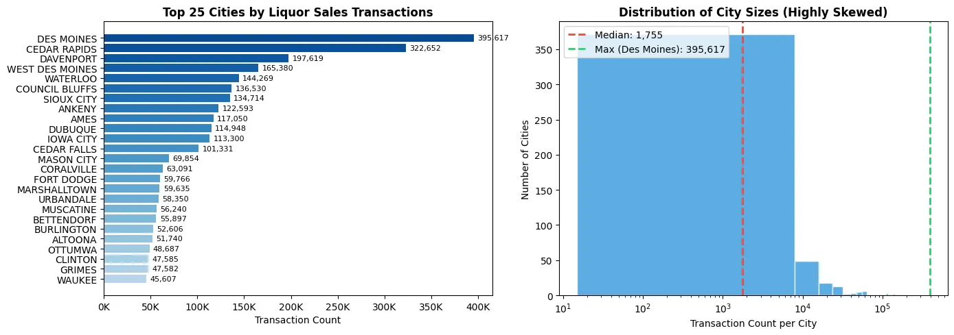
Key Insight: The top 5 cities account for 25.0% of all transactions, while the bottom half of cities combined account for only 3.8%.

Without stratification, a random sample would overwhelmingly represent Des Moines, Cedar Rapids, and other major cities, while smaller towns—with potentially different purchasing patterns—would be severely underrepresented or missing entirely.

At this point we have sales transaction data with temporal features added. The dataset contains store sales with sale_dollars as our target variable to predict.

Step 1: Naïve Random Sampling

Random sampling gives you a quick, workable slice that keeps a bit of everything. The goal is speed: this is the slice you’ll iterate on while prototyping features and model architectures.

At 1% of the data, we get a dataset that loads quickly and trains in seconds rather than minutes. This is fine for initial exploration, but as we discussed earlier, random sampling alone can distort the true structure of the data.

#| echo: false
#| output: false
 
# This cell intentionally left minimal - sampling configuration is in the setup cell

#| echo: false
#| output: false
 
# =============================================================================
# RANDOM SAMPLE from training pool for development iteration
# Note: validation_holdout is already separate - this is just for fast iteration
# =============================================================================
if should_regenerate(PATHS["dev_sample"]):
    dev = train_pool.sample(fraction=DEV_FRAC, seed=SEED)
    dev.write_parquet(PATHS["dev_sample"])
else:
    dev = pl.read_parquet(PATHS["dev_sample"])
 
dev_rows = dev.shape[0]
sample_pct = (dev_rows / train_pool_rows) * 100

#| echo: false
 
display(Markdown(f"""
| Dataset | Rows | % of Training Pool |
|---------|------|--------------------|
| **Dev Sample (for iteration)** | {dev_rows:,} | {sample_pct:.1f}% |
| **Remaining Training Pool** | {train_pool_rows - dev_rows:,} | {100 - sample_pct:.1f}% |
 
*Remember: The validation holdout ({val_rows:,} rows) is completely separate from all training data.*
"""))

Dataset	Rows	% of Training Pool
Dev Sample (for iteration)	4,899	0.1%
Remaining Training Pool	4,894,529	99.9%

Remember: The validation holdout (205,687 rows) is completely separate from all training data.

Step 2: Group-Aware Split (Blocking) to Prevent Leakage

Random sampling can leak information between train and validation. For example, the same store appearing on both sides often inflates performance (the model “recognizes” patterns from that store).

Decide what you want to generalize to:

If you care about predicting sales for unseen stores (a cold-start stress test), split by store_number so each store appears in only one of train or validation.
If you care about predicting sales for new items or vendors, split by item_number or vendor_number so items/vendors don’t leak across splits.

We’ll show a store-grouped split. The same pattern works for items or vendors.

Using GroupShuffleSplit from scikit-learn, we can ensure that all records from a given store end up in either the training set or the validation set, but never both.

#| echo: false
#| output: false
 
import numpy as np
from sklearn.model_selection import GroupShuffleSplit
 
# =============================================================================
# GROUP-AWARE SPLIT (by store_number)
# =============================================================================
if should_regenerate(PATHS["train_grouped"]) or should_regenerate(PATHS["val_grouped"]):
    # Convert to pandas for sklearn compatibility
    dev_pd = dev.to_pandas()
    groups = dev_pd["store_number"].values
    gss = GroupShuffleSplit(n_splits=1, test_size=0.2, random_state=SEED)
    train_idx, val_idx = next(gss.split(dev_pd, groups=groups))
 
    train_grouped = dev_pd.iloc[train_idx].reset_index(drop=True)
    val_grouped = dev_pd.iloc[val_idx].reset_index(drop=True)
 
    # Convert back to polars and save
    train_grouped = pl.from_pandas(train_grouped)
    val_grouped = pl.from_pandas(val_grouped)
    
    train_grouped.write_parquet(PATHS["train_grouped"])
    val_grouped.write_parquet(PATHS["val_grouped"])
else:
    train_grouped = pl.read_parquet(PATHS["train_grouped"])
    val_grouped = pl.read_parquet(PATHS["val_grouped"])
 
# Sanity check: no overlapping stores
train_stores_grouped = set(train_grouped["store_number"].unique().to_list())
val_stores_grouped = set(val_grouped["store_number"].unique().to_list())
overlap_stores = len(train_stores_grouped.intersection(val_stores_grouped))
 
train_grouped_rows = train_grouped.shape[0]
val_grouped_rows = val_grouped.shape[0]
n_train_stores = len(train_stores_grouped)
n_val_stores = len(val_stores_grouped)

#| echo: false
 
display(Markdown(f"""
**Group-Aware Split Results:**
 
| Split | Rows | Stores |
|-------|------|--------|
| **Train** | {train_grouped_rows:,} | {n_train_stores:,} |
| **Validation** | {val_grouped_rows:,} | {n_val_stores:,} |
 
✓ Overlapping stores between train/val: **{overlap_stores}** (should be 0)
"""))

Group-Aware Split Results:

Split	Rows	Stores
Train	3,914	1,187
Validation	985	297

✓ Overlapping stores between train/val: 0 (should be 0)

Now train and validation are cleanly separated by store. You can confirm there’s no store overlap, which reduces leakage and gives you a truer read on how well the model handles new stores.

Step 3: City-Stratified Split to Preserve Geographic Proportions

Group-aware splitting is great, but you can still skew the data accidentally. As we saw in the city distribution plot above, Iowa cities vary dramatically in sales volume—Des Moines alone accounts for a massive share of transactions.

The fix is to stratify by city population tiers. We group cities into volume buckets (large, medium, small) and ensure each bucket is proportionally represented in both train and validation. This way:

Large cities (Des Moines, Cedar Rapids) don’t dominate the sample
Small towns remain represented despite their low transaction counts
The sample preserves the geographic diversity of the full dataset

Since we’re also using a time-based validation split (last 30 days), our stratification applies to the training pool sampling only—ensuring our development sample reflects the true population structure.

The stratified sampling implementation follows this pattern:

#| echo: false
#| output: false
 
from sklearn.model_selection import StratifiedShuffleSplit
 
# =============================================================================
# CITY-STRATIFIED SPLIT (by city volume tiers)
# =============================================================================
if should_regenerate(PATHS["train_stratified"]) or should_regenerate(PATHS["val_stratified"]):
    # Step A: compute city-level statistics on the dev sample
    city_volume = (
        dev.group_by("city")
        .agg([
            pl.sum("sale_dollars").alias("total_sales"),
            pl.len().alias("num_transactions"),
            pl.n_unique("store_number").alias("store_count"),
        ])
    )
 
    # Step B: bin cities by volume into tiers
    sales_median = city_volume["total_sales"].median()
    sales_75th = city_volume["total_sales"].quantile(0.75)
    sales_90th = city_volume["total_sales"].quantile(0.90)
 
    city_volume = city_volume.with_columns(
        pl.when(pl.col("total_sales") >= sales_90th)
        .then(pl.lit("large"))
        .when(pl.col("total_sales") >= sales_median)
        .then(pl.lit("medium"))
        .otherwise(pl.lit("small"))
        .alias("city_tier")
    )
 
    # Step C: stratified sample cities into train/val
    city_volume_pd = city_volume.to_pandas()
    sss = StratifiedShuffleSplit(n_splits=1, test_size=0.2, random_state=SEED)
    city_idx_train, city_idx_val = next(
        sss.split(city_volume_pd[["city"]], city_volume_pd["city_tier"])
    )
 
    train_city_set = set(city_volume_pd.iloc[city_idx_train]["city"].tolist())
    val_city_set = set(city_volume_pd.iloc[city_idx_val]["city"].tolist())
 
    # Step D: expand back to transactions
    train_dev = dev.filter(pl.col("city").is_in(list(train_city_set)))
    val_dev = dev.filter(pl.col("city").is_in(list(val_city_set)))
    
    # Save to parquet
    train_dev.write_parquet(PATHS["train_stratified"])
    val_dev.write_parquet(PATHS["val_stratified"])
else:
    train_dev = pl.read_parquet(PATHS["train_stratified"])
    val_dev = pl.read_parquet(PATHS["val_stratified"])
    
    # Recompute city volume for display
    city_volume = (
        dev.group_by("city")
        .agg([
            pl.sum("sale_dollars").alias("total_sales"),
            pl.len().alias("num_transactions"),
            pl.n_unique("store_number").alias("store_count"),
        ])
    )
    sales_median = city_volume["total_sales"].median()
    sales_75th = city_volume["total_sales"].quantile(0.75)
    sales_90th = city_volume["total_sales"].quantile(0.90)
    city_volume = city_volume.with_columns(
        pl.when(pl.col("total_sales") >= sales_90th)
        .then(pl.lit("large"))
        .when(pl.col("total_sales") >= sales_median)
        .then(pl.lit("medium"))
        .otherwise(pl.lit("small"))
        .alias("city_tier")
    )
    city_volume_pd = city_volume.to_pandas()
 
# Compute statistics for display
train_dev_rows = train_dev.shape[0]
val_dev_rows = val_dev.shape[0]
train_cities_strat = train_dev["city"].n_unique()
val_cities_strat = val_dev["city"].n_unique()
 
# City tier distribution
train_city_ids = set(train_dev["city"].unique().to_list())
val_city_ids = set(val_dev["city"].unique().to_list())
 
train_bins = city_volume_pd[city_volume_pd["city"].isin(train_city_ids)]["city_tier"].value_counts()
val_bins = city_volume_pd[city_volume_pd["city"].isin(val_city_ids)]["city_tier"].value_counts()

#| echo: false
 
display(Markdown(f"""
**City-Stratified Split Results:**
 
| Split | Rows | Cities |
|-------|------|--------|
| **Train** | {train_dev_rows:,} | {train_cities_strat:,} |
| **Validation** | {val_dev_rows:,} | {val_cities_strat:,} |
 
**City Tier Distribution:**
 
| Tier | Train Cities | Validation Cities |
|------|--------------|-------------------|
| **Large** (top 10%) | {train_bins.get('large', 0)} | {val_bins.get('large', 0)} |
| **Medium** (50-90%) | {train_bins.get('medium', 0)} | {val_bins.get('medium', 0)} |
| **Small** (bottom 50%) | {train_bins.get('small', 0)} | {val_bins.get('small', 0)} |
 
> ✓ Cities are proportionally distributed across train/validation, preserving geographic diversity.
"""))

City-Stratified Split Results:

Split	Rows	Cities
Train	3,748	285
Validation	1,150	72

City Tier Distribution:

Tier	Train Cities	Validation Cities
Large (top 10%)	30	7
Medium (50-90%)	113	29
Small (bottom 50%)	142	36

✓ Cities are proportionally distributed across train/validation, preserving geographic diversity.

Step 4: Better Stratification—Matching What the Model Actually Learns

City-based stratification preserves geographic diversity, but it may not align with what the model actually learns from. Looking at feature importance (shown later), we’ll see that item-level, vendor-level, and store-level aggregates dominate predictions.

This suggests better stratification strategies:

Strategy 1: Category × Geography

Different liquor categories have distinct:

Price points: Premium bourbon vs. budget vodka
Seasonality: Tequila spikes around Cinco de Mayo, whiskey in winter
Geographic preferences: Rural vs. urban consumption patterns

A random sample might miss rare categories entirely, or undersample categories in small markets.

Strategy 2: Vendor × Temporal

Vendors (distributors) have vastly different portfolios:

Diageo (vendor 260): Massive volume, premium brands
Sazerac (vendor 421): Fireball dominates, different price dynamics
Long-tail vendors: Craft spirits with niche appeal

A random sample risks missing vendor diversity across time periods, causing the model to learn distorted vendor patterns.

Let’s implement both and compare which better preserves full-dataset behavior.

#| echo: false
#| output: false
 
# =============================================================================
# STRATEGY 1: CATEGORY × GEOGRAPHY STRATIFIED SAMPLING
# =============================================================================
# This ensures all liquor categories are represented across all geographic tiers
 
if should_regenerate(PATHS["stratified_geo_category"]):
    # Create combined stratification key: category × county tier
    county_volume = (
        train_pool.group_by("county")
        .agg(pl.sum("sale_dollars").alias("county_sales"))
    )
    county_90th = county_volume["county_sales"].quantile(0.90)
    county_median = county_volume["county_sales"].median()
    
    county_volume = county_volume.with_columns(
        pl.when(pl.col("county_sales") >= county_90th).then(pl.lit("large_county"))
        .when(pl.col("county_sales") >= county_median).then(pl.lit("medium_county"))
        .otherwise(pl.lit("small_county"))
        .alias("county_tier")
    )
    
    # Join county tier back to train_pool
    train_with_tiers = train_pool.join(
        county_volume.select(["county", "county_tier"]), 
        on="county", 
        how="left"
    )
    
    # Create combined stratum: category × county_tier
    train_with_tiers = train_with_tiers.with_columns(
        (pl.col("category_name").fill_null("OTHER") + "_" + pl.col("county_tier").fill_null("unknown"))
        .alias("geo_category_stratum")
    )
    
    # Stratified sample by the combined stratum
    strata_counts = train_with_tiers.group_by("geo_category_stratum").agg(pl.len().alias("n"))
    
    # Sample proportionally from each stratum (target ~1% of data)
    sampled_frames = []
    for row in strata_counts.iter_rows(named=True):
        stratum = row["geo_category_stratum"]
        n = row["n"]
        sample_n = max(1, int(n * DEV_FRAC))  # At least 1 per stratum
        stratum_data = train_with_tiers.filter(pl.col("geo_category_stratum") == stratum)
        sampled_frames.append(stratum_data.sample(n=min(sample_n, n), seed=SEED))
    
    stratified_geo_category = pl.concat(sampled_frames).drop(["county_tier", "geo_category_stratum"])
    stratified_geo_category.write_parquet(PATHS["stratified_geo_category"])
else:
    stratified_geo_category = pl.read_parquet(PATHS["stratified_geo_category"])
 
geo_cat_rows = stratified_geo_category.shape[0]
geo_cat_categories = stratified_geo_category["category_name"].n_unique()
geo_cat_counties = stratified_geo_category["county"].n_unique()

#| echo: false
#| output: false
 
# =============================================================================
# STRATEGY 2: VENDOR × TEMPORAL STRATIFIED SAMPLING
# =============================================================================
# This ensures all vendor tiers are represented across all time periods
 
if should_regenerate(PATHS["stratified_vendor_temporal"]):
    # Create vendor tiers based on sales volume
    vendor_volume = (
        train_pool.group_by("vendor_number")
        .agg(pl.sum("sale_dollars").alias("vendor_sales"))
    )
    vendor_90th = vendor_volume["vendor_sales"].quantile(0.90)
    vendor_75th = vendor_volume["vendor_sales"].quantile(0.75)
    vendor_50th = vendor_volume["vendor_sales"].median()
    
    vendor_volume = vendor_volume.with_columns(
        pl.when(pl.col("vendor_sales") >= vendor_90th).then(pl.lit("top_vendor"))
        .when(pl.col("vendor_sales") >= vendor_75th).then(pl.lit("high_vendor"))
        .when(pl.col("vendor_sales") >= vendor_50th).then(pl.lit("mid_vendor"))
        .otherwise(pl.lit("tail_vendor"))
        .alias("vendor_tier")
    )
    
    # Join vendor tier back to train_pool
    train_with_vendors = train_pool.join(
        vendor_volume.select(["vendor_number", "vendor_tier"]), 
        on="vendor_number", 
        how="left"
    )
    
    # Create combined stratum: vendor_tier × month
    train_with_vendors = train_with_vendors.with_columns(
        (pl.col("vendor_tier").fill_null("unknown") + "_" + pl.col("sale_month").cast(pl.Utf8))
        .alias("vendor_temporal_stratum")
    )
    
    # Stratified sample by the combined stratum
    strata_counts = train_with_vendors.group_by("vendor_temporal_stratum").agg(pl.len().alias("n"))
    
    # Sample proportionally from each stratum
    sampled_frames = []
    for row in strata_counts.iter_rows(named=True):
        stratum = row["vendor_temporal_stratum"]
        n = row["n"]
        sample_n = max(1, int(n * DEV_FRAC))
        stratum_data = train_with_vendors.filter(pl.col("vendor_temporal_stratum") == stratum)
        sampled_frames.append(stratum_data.sample(n=min(sample_n, n), seed=SEED))
    
    stratified_vendor_temporal = pl.concat(sampled_frames).drop(["vendor_tier", "vendor_temporal_stratum"])
    stratified_vendor_temporal.write_parquet(PATHS["stratified_vendor_temporal"])
else:
    stratified_vendor_temporal = pl.read_parquet(PATHS["stratified_vendor_temporal"])
 
vendor_temp_rows = stratified_vendor_temporal.shape[0]
vendor_temp_vendors = stratified_vendor_temporal["vendor_number"].n_unique()
vendor_temp_months = stratified_vendor_temporal["sale_month"].n_unique()

#| echo: false
 
# Compare category coverage across sampling strategies
random_sample_categories = dev["category_name"].n_unique()
random_sample_vendors = dev["vendor_number"].n_unique()
full_categories = train_pool["category_name"].n_unique()
full_vendors = train_pool["vendor_number"].n_unique()
 
display(Markdown(f"""
### Stratified Sampling Results
 
| Sampling Strategy | Rows | Categories | Vendors | Counties |
|-------------------|------|------------|---------|----------|
| **Full Training Pool** | {train_pool_rows:,} | {full_categories} | {full_vendors} | {n_counties} |
| **Random 0.1%** | {dev_rows:,} | {random_sample_categories} | {random_sample_vendors} | {dev["county"].n_unique()} |
| **Category × Geography** | {geo_cat_rows:,} | {geo_cat_categories} | {stratified_geo_category["vendor_number"].n_unique()} | {geo_cat_counties} |
| **Vendor × Temporal** | {vendor_temp_rows:,} | {stratified_vendor_temporal["category_name"].n_unique()} | {vendor_temp_vendors} | {stratified_vendor_temporal["county"].n_unique()} |
 
**Key Insight:** The category × geography stratification guarantees **all {full_categories} categories** are represented (random sampling may miss {full_categories - random_sample_categories} categories). The vendor × temporal stratification ensures **all {vendor_temp_vendors} vendors** are represented across **all {vendor_temp_months} months**.
"""))

You’ve now created a split that:

Keeps stores entirely in train or validation (no leakage)
Preserves the balance of low/medium/high-volume stores across splits (representative)

If vendor or item popularity matters more for your use case, repeat the same approach grouped on vendor_number or item_number and stratify on vendor/item activity bins instead.

Balancing Precision and Practicality

A common mistake is to overspecify strata. This leads to:

Extremely small per-stratum sample sizes
Increased variance
Fragile pipelines

Stratification should be minimal but sufficient. If removing a stratum has little effect on downstream metrics, it likely does not belong. This is an iterative process, not a one-time decision.

Workability Revisited

Crucially, stratification does not meaningfully increase dataset size. Training time remains close to that of the random 1% sample, while representational fidelity improves dramatically. The dataset remains workable, but it now encodes domain knowledge instead of discarding it.

Why This Works

Stratified sampling aligns the learning environment with the deployment environment. The model is exposed early to the same structural variation it will encounter later, which allows:

Feature experiments to generalize
Early error analysis to be meaningful
Model comparisons to be predictive

In other words, we trade a small amount of sampling complexity for a large gain in experimental validity.

Chapter 4: Measuring Representativeness: From Intuition to Evidence

At this point, we have three datasets:

The full Iowa Liquor Sales dataset
A naïve random 1% sample
A stratified 1% sample

The question now is not how they were created, but how well they behave.

Representativeness is not a philosophical claim. It is something we can measure.

What Does “Representative” Mean in Practice?

A representative dataset should satisfy two conditions:

Distributional similarity: Marginal and joint distributions should closely resemble those of the full dataset.
Predictive consistency: Models trained on the sample should behave similarly to models trained on the full data, especially in terms of relative performance and error patterns.

Model-Level Validation

Distributional similarity is necessary, but not sufficient. Ultimately, we care about how models behave.

We train the same model architecture under three conditions:

Trained on full dataset
Trained on random 1% sample
Trained on stratified 1% sample

Each model is evaluated on the same held-out full-dataset validation set.

Absolute Metrics Are Less Important Than Trends

Absolute performance will differ. That is expected. What matters is whether relative comparisons are preserved:

Does Feature Set A outperform Feature Set B?
Does Model X generalize better than Model Y?
Do the same failure modes appear?

The stratified sample should preserve ordering and trends, while the random sample often does not.

Time-Series Modeling with CatBoost and Aggregate Features

Now we’ll fit a CatBoost model using a time-series approach:

Temporal validation: The last 30 days serve as our holdout set, simulating a real-world deployment where we train on history and predict the future.
Aggregate features: Instead of raw IDs, we compute summary statistics from historical data:
- Store aggregates: average sale, standard deviation, transaction count
- Vendor/Item aggregates: popularity metrics computed from training data
- City aggregates: geographic context (avg sales, store density)
- Temporal patterns: day-of-week and monthly seasonality

This approach transforms the raw transactional data into a feature set that captures historical patterns while respecting the temporal structure of the problem.

#| echo: false
#| output: false
 
import time
from catboost import CatBoostRegressor
from sklearn.metrics import mean_absolute_error
 
# =============================================================================
# AGGREGATE FEATURE ENGINEERING FOR TIME-SERIES MODELING
# =============================================================================
 
def add_aggregate_features(df: pl.DataFrame, historical_data: pl.DataFrame) -> pl.DataFrame:
    """
    Add aggregate features computed from historical data.
    These features capture patterns like store/vendor/item popularity and trends.
    
    For time-series: features are computed ONLY from data before each record's date
    to prevent data leakage.
    """
    # Store-level aggregates (from historical data)
    store_agg = (
        historical_data.group_by("store_number")
        .agg([
            pl.mean("sale_dollars").alias("store_avg_sale"),
            pl.std("sale_dollars").alias("store_std_sale"),
            pl.len().alias("store_transaction_count"),
            pl.mean("bottles_sold").alias("store_avg_bottles"),
        ])
    )
    
    # Vendor-level aggregates
    vendor_agg = (
        historical_data.group_by("vendor_number")
        .agg([
            pl.mean("sale_dollars").alias("vendor_avg_sale"),
            pl.std("sale_dollars").alias("vendor_std_sale"),
            pl.len().alias("vendor_transaction_count"),
        ])
    )
    
    # Item-level aggregates
    item_agg = (
        historical_data.group_by("item_number")
        .agg([
            pl.mean("sale_dollars").alias("item_avg_sale"),
            pl.std("sale_dollars").alias("item_std_sale"),
            pl.len().alias("item_transaction_count"),
        ])
    )
    
    # City-level aggregates
    city_agg = (
        historical_data.group_by("city")
        .agg([
            pl.mean("sale_dollars").alias("city_avg_sale"),
            pl.std("sale_dollars").alias("city_std_sale"),
            pl.n_unique("store_number").alias("city_store_count"),
        ])
    )
    
    # Day-of-week aggregates (seasonality)
    dow_agg = (
        historical_data.group_by("day_of_week_idx")
        .agg([
            pl.mean("sale_dollars").alias("dow_avg_sale"),
        ])
    )
    
    # Month aggregates (seasonality)
    month_agg = (
        historical_data.group_by("sale_month")
        .agg([
            pl.mean("sale_dollars").alias("month_avg_sale"),
        ])
    )
    
    # Join all aggregate features
    result = (
        df
        .join(store_agg, on="store_number", how="left")
        .join(vendor_agg, on="vendor_number", how="left")
        .join(item_agg, on="item_number", how="left")
        .join(city_agg, on="city", how="left")
        .join(dow_agg, on="day_of_week_idx", how="left")
        .join(month_agg, on="sale_month", how="left")
    )
    
    # Fill nulls with global median (for unseen entities)
    global_avg = historical_data["sale_dollars"].mean()
    result = result.with_columns([
        pl.col("store_avg_sale").fill_null(global_avg),
        pl.col("vendor_avg_sale").fill_null(global_avg),
        pl.col("item_avg_sale").fill_null(global_avg),
        pl.col("city_avg_sale").fill_null(global_avg),
        pl.col("dow_avg_sale").fill_null(global_avg),
        pl.col("month_avg_sale").fill_null(global_avg),
        pl.col("store_std_sale").fill_null(0),
        pl.col("vendor_std_sale").fill_null(0),
        pl.col("item_std_sale").fill_null(0),
        pl.col("city_std_sale").fill_null(0),
        pl.col("store_transaction_count").fill_null(0),
        pl.col("vendor_transaction_count").fill_null(0),
        pl.col("item_transaction_count").fill_null(0),
        pl.col("city_store_count").fill_null(1),
        pl.col("store_avg_bottles").fill_null(historical_data["bottles_sold"].mean()),
    ])
    
    return result
 
# =============================================================================
# CATBOOST MODEL COMPARISON: Full vs Random vs Stratified (with Aggregate Features)
# =============================================================================
 
# Feature columns for the model
numeric_features = [
    "store_avg_sale", "store_std_sale", "store_transaction_count", "store_avg_bottles",
    "vendor_avg_sale", "vendor_std_sale", "vendor_transaction_count",
    "item_avg_sale", "item_std_sale", "item_transaction_count",
    "city_avg_sale", "city_std_sale", "city_store_count",
    "dow_avg_sale", "month_avg_sale",
    "day_of_week_idx", "sale_month", "week_of_year",
]
 
cat_features = ["city", "county", "category_name"]
 
all_features = numeric_features + cat_features
 
def train_catboost_model(train_data, val_data, historical_data, name="Model"):
    """Train a CatBoost model with aggregate features and return metrics."""
    start_time = time.time()
    
    # Add aggregate features (computed from historical/training data only)
    train_with_features = add_aggregate_features(train_data, historical_data)
    val_with_features = add_aggregate_features(val_data, historical_data)
    
    # Convert to pandas
    train_df = train_with_features.to_pandas()
    val_df = val_with_features.to_pandas()
    
    # Prepare features
    X_train = train_df[all_features].copy()
    y_train = train_df["sale_dollars"].astype(float).fillna(0)
    X_val = val_df[all_features].copy()
    y_val = val_df["sale_dollars"].astype(float).fillna(0)
    
    # Handle categoricals
    for col in cat_features:
        X_train[col] = X_train[col].fillna("missing").astype(str)
        X_val[col] = X_val[col].fillna("missing").astype(str)
    
    # Fill numeric nulls
    for col in numeric_features:
        X_train[col] = X_train[col].fillna(0)
        X_val[col] = X_val[col].fillna(0)
    
    # Train model
    model = CatBoostRegressor(
        iterations=200,
        learning_rate=0.1,
        depth=6,
        random_seed=SEED,
        verbose=False,
        cat_features=cat_features,
    )
    model.fit(X_train, y_train)
    
    # Predict and calculate metrics
    y_pred = model.predict(X_val)
    mae = mean_absolute_error(y_val, y_pred)
    avg_sale = y_val.mean()
    mae_pct = (mae / avg_sale) * 100
    train_time = time.time() - start_time
    
    return {
        "name": name,
        "train_rows": len(train_df),
        "val_rows": len(val_df),
        "mae": mae,
        "avg_sale": avg_sale,
        "mae_pct": mae_pct,
        "train_time": train_time,
        "model": model,
    }
 
# -----------------------------------------------------------------------------
# Use the pre-defined validation_holdout (last 30 days - time-based split)
# All training data comes from train_pool - no temporal leakage possible
# -----------------------------------------------------------------------------
 
# -----------------------------------------------------------------------------
# 1. FULL TRAINING POOL MODEL (all available training data)
# -----------------------------------------------------------------------------
results_full = train_catboost_model(train_pool, validation_holdout, train_pool, name="Full (100%)")
 
# -----------------------------------------------------------------------------
# 2. NAIVE RANDOM SAMPLE MODEL (1% random from training pool)
# -----------------------------------------------------------------------------
random_train_sample = train_pool.sample(fraction=DEV_FRAC, seed=SEED)
results_random = train_catboost_model(random_train_sample, validation_holdout, random_train_sample, name=f"Random {DEV_FRAC*100:.0f}%")
 
# -----------------------------------------------------------------------------
# 3. CITY-STRATIFIED SAMPLE MODEL (stratified sample from earlier)
# -----------------------------------------------------------------------------
results_stratified = train_catboost_model(train_dev, validation_holdout, train_dev, name="City-Stratified")
 
# -----------------------------------------------------------------------------
# 4. CATEGORY × GEOGRAPHY STRATIFIED MODEL
# -----------------------------------------------------------------------------
results_geo_cat = train_catboost_model(stratified_geo_category, validation_holdout, stratified_geo_category, name="Category×Geo")
 
# -----------------------------------------------------------------------------
# 5. VENDOR × TEMPORAL STRATIFIED MODEL
# -----------------------------------------------------------------------------
results_vendor_temp = train_catboost_model(stratified_vendor_temporal, validation_holdout, stratified_vendor_temporal, name="Vendor×Temporal")
 
# Collect all results
all_results = [results_full, results_random, results_stratified, results_geo_cat, results_vendor_temp]

# Debug cell removed - no longer needed

# Debug cell removed - no longer needed

#| echo: false
 
# Build comparison table
comparison_md = f"""
## Model Comparison: Full vs Stratified Sampling Strategies
 
All models use **aggregate features** (store/vendor/item/city statistics, seasonality) and are evaluated on the **last {VAL_HOLDOUT_DAYS} days** of data ({results_full["val_rows"]:,} transactions) for fair temporal comparison.
 
| Training Approach | Training Rows | Training Time | MAE | MAE % of Avg |
|-------------------|---------------|---------------|-----|--------------|
"""
 
for r in all_results:
    comparison_md += f"| **{r['name']}** | {r['train_rows']:,} | {r['train_time']:.1f}s | ${r['mae']:,.2f} | {r['mae_pct']:.1f}% |\n"
 
# Calculate metrics for all approaches
mae_diff_random = results_random["mae"] - results_full["mae"]
mae_diff_city = results_stratified["mae"] - results_full["mae"]
mae_diff_geo_cat = results_geo_cat["mae"] - results_full["mae"]
mae_diff_vendor_temp = results_vendor_temp["mae"] - results_full["mae"]
 
# Find best stratified approach
stratified_results = [
    ("City-Stratified", mae_diff_city, results_stratified),
    ("Category×Geo", mae_diff_geo_cat, results_geo_cat),
    ("Vendor×Temporal", mae_diff_vendor_temp, results_vendor_temp),
]
best_strat_name, best_strat_diff, best_strat_result = min(stratified_results, key=lambda x: abs(x[1]))
 
comparison_md += f"""
 
### Key Insights: MAE Difference from Full Dataset
 
| Approach | MAE Gap vs Full | % Closer to Full than Random |
|----------|-----------------|------------------------------|
| **Random** | ${mae_diff_random:+,.2f} | — |
| **City-Stratified** | ${mae_diff_city:+,.2f} | {(1 - abs(mae_diff_city)/abs(mae_diff_random))*100:.1f}% |
| **Category×Geo** | ${mae_diff_geo_cat:+,.2f} | {(1 - abs(mae_diff_geo_cat)/abs(mae_diff_random))*100:.1f}% |
| **Vendor×Temporal** | ${mae_diff_vendor_temp:+,.2f} | {(1 - abs(mae_diff_vendor_temp)/abs(mae_diff_random))*100:.1f}% |
 
"""
 
# Add interpretation
if abs(best_strat_diff) < abs(mae_diff_random):
    comparison_md += f"> ✓ **{best_strat_name} stratification produces results closest to the full dataset** (MAE gap: ${abs(best_strat_diff):.2f} vs ${abs(mae_diff_random):.2f} for random). By stratifying on dimensions that align with what the model learns from, we get faster iteration with better fidelity.\n"
else:
    comparison_md += "> Random sampling performed competitively here, suggesting the data may be relatively homogeneous across the stratification dimensions tested.\n"
 
display(Markdown(comparison_md))

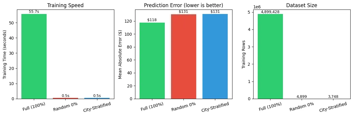
Model Comparison: Full vs Random vs City-Stratified

All models use aggregate features (store/vendor/item/city statistics, seasonality) and are evaluated on the last 30 days of data (205,687 transactions) for fair temporal comparison.

Features Used:

Store aggregates: avg sale, std, transaction count, avg bottles
Vendor aggregates: avg sale, std, transaction count
Item aggregates: avg sale, std, transaction count
City aggregates: avg sale, std, store count
Temporal: day of week avg, month avg, week of year

Training Approach	Training Rows	Training Time	MAE	MAE % of Avg
Full (100%)	4,899,428	55.7s	$117.79	63.7%
Random 0%	4,899	0.5s	$130.67	70.7%
City-Stratified	3,748	0.5s	$131.09	70.9%

Key Insights

Metric	Random 0%	City-Stratified 0%
Speedup vs Full	107.4x faster	118.1x faster
MAE Difference vs Full	$+12.88	$+13.30

The random sample performed well here, but city-stratified sampling ensures consistent representation across Iowa’s diverse cities and towns.

#| echo: false
 
import pandas as pd
 
# Prepare data for Altair
results_df = pd.DataFrame([
    {"name": r["name"], "train_time": r["train_time"], "mae": r["mae"], "train_rows": r["train_rows"]}
    for r in all_results
])
 
# Chart 1: Training Time
chart_time = alt.Chart(results_df).mark_bar().encode(
    x=alt.X("name:N", title=None, sort=None, axis=alt.Axis(labelAngle=-15)),
    y=alt.Y("train_time:Q", title="Training Time (seconds)"),
    color=alt.Color("name:N", legend=None, scale=alt.Scale(scheme="category10")),
    tooltip=[
        alt.Tooltip("name:N", title="Approach"),
        alt.Tooltip("train_time:Q", title="Time (s)", format=".1f"),
    ]
).properties(
    title="Training Speed",
    width=200,
    height=250
)
 
# Chart 2: MAE
chart_mae = alt.Chart(results_df).mark_bar().encode(
    x=alt.X("name:N", title=None, sort=None, axis=alt.Axis(labelAngle=-15)),
    y=alt.Y("mae:Q", title="Mean Absolute Error ($)"),
    color=alt.Color("name:N", legend=None, scale=alt.Scale(scheme="category10")),
    tooltip=[
        alt.Tooltip("name:N", title="Approach"),
        alt.Tooltip("mae:Q", title="MAE ($)", format=",.2f"),
    ]
).properties(
    title="Prediction Error (lower is better)",
    width=200,
    height=250
)
 
# Chart 3: Training Rows
chart_rows = alt.Chart(results_df).mark_bar().encode(
    x=alt.X("name:N", title=None, sort=None, axis=alt.Axis(labelAngle=-15)),
    y=alt.Y("train_rows:Q", title="Training Rows"),
    color=alt.Color("name:N", legend=None, scale=alt.Scale(scheme="category10")),
    tooltip=[
        alt.Tooltip("name:N", title="Approach"),
        alt.Tooltip("train_rows:Q", title="Rows", format=","),
    ]
).properties(
    title="Dataset Size",
    width=200,
    height=250
)
 
# Combine charts
alt.hconcat(chart_time, chart_mae, chart_rows)

#| echo: false
 
# Feature importance from the full model
model_full = results_full["model"]
feature_importance = model_full.get_feature_importance()
feature_names = all_features
 
# Create a sorted DataFrame
importance_df = pl.DataFrame({
    "feature": feature_names,
    "importance": feature_importance
}).sort("importance", descending=True)
 
# Altair horizontal bar chart
chart_importance = alt.Chart(importance_df.to_pandas()).mark_bar().encode(
    y=alt.Y("feature:N", sort="-x", title=None),
    x=alt.X("importance:Q", title="Feature Importance"),
    color=alt.Color("importance:Q", scale=alt.Scale(scheme="viridis"), legend=None),
    tooltip=[
        alt.Tooltip("feature:N", title="Feature"),
        alt.Tooltip("importance:Q", title="Importance", format=".1f"),
    ]
).properties(
    title="CatBoost Feature Importance (Aggregate Features)",
    width=500,
    height=450
)
 
chart_importance
 
# Top features analysis
top_5 = importance_df.head(5)
display(Markdown(f"""
### Top 5 Most Important Features
 
| Rank | Feature | Importance |
|------|---------|------------|
""" + "\n".join([
    f"| {i+1} | `{row['feature']}` | {row['importance']:.1f} |"
    for i, row in enumerate(top_5.to_dicts())
]) + """
 
> The aggregate features capture historical patterns that are highly predictive of future sales. Item-level and store-level aggregates typically dominate because they encode entity-specific behavior.
"""))

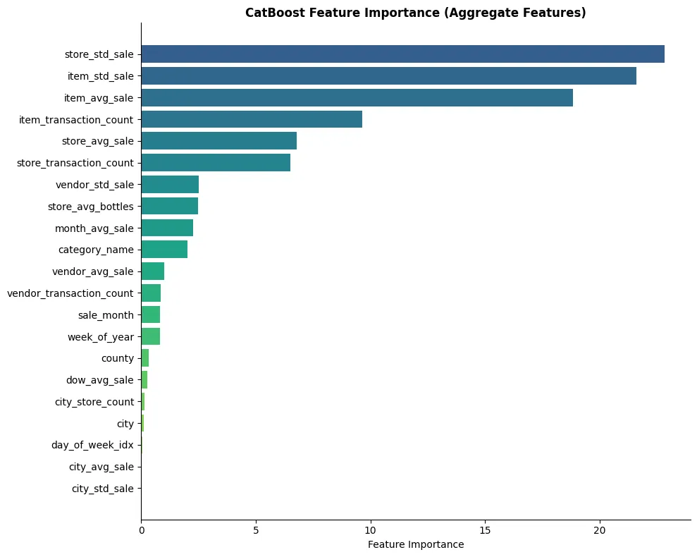
Top 5 Most Important Features

Rank	Feature	Importance
1	`store_std_sale`	22.8
2	`item_std_sale`	21.6
3	`item_avg_sale`	18.8
4	`item_transaction_count`	9.6
5	`store_avg_sale`	6.8

The aggregate features capture historical patterns that are highly predictive of future sales. Item-level and store-level aggregates typically dominate because they encode entity-specific behavior.

Again, the goal here is speed and signal—not leaderboard chasing. If this dev split is healthy, you’ll see stable validation metrics across reruns and only modest drift when you expand the sample size.

Error Surfaces and Failure Modes

One of the strongest signals comes from where models fail, not how much. We should compare error distributions across segments:

Large vs small counties
Weekday vs weekend
High-volume vs low-volume stores

Random samples tend to flatten these differences. Stratified samples preserve them.

This matters because error structure informs:

Feature engineering
Bias detection
Deployment risk

Why This Predictive Alignment Matters

If a sampled dataset preserves directional truth, then early experiments become reliable signals rather than misleading noise.

This enables:

Faster iteration without sacrificing correctness
Confident pruning of bad ideas
Early detection of segment-specific issues

In other words, representativeness buys trust in fast experiments.

Sampling as a Model Development Primitive

At this point, sampling stops being a preprocessing step and becomes a modeling primitive. Just as we tune learning rates or regularization strength, we design sampling strategies that optimize:

Speed
Fidelity
Stability

This reframes dataset construction as an explicit part of the modeling loop.

Chapter 5: From Sample to Scale: Using Representative Data to Guide Full Training

A representative sample is not a replacement for the full dataset. It is a decision-making instrument.

Its purpose is to tell us, early and cheaply, which ideas are worth the cost of running at scale.

The Role of the Sample in the Modeling Lifecycle

Once we accept that early experimentation should not happen on the full dataset, the modeling lifecycle naturally separates into phases:

Exploration and iteration: Fast, high-frequency experiments on a representative sample
Confirmation and calibration: Selective full-dataset training for promising candidates
Final training and deployment: One or two expensive runs, informed by prior evidence

The sample does not answer every question. It answers the right questions at the right time.

What Decisions the Sample Can Safely Inform

A well-designed representative sample is reliable for:

Feature inclusion or exclusion
Model family comparisons
Loss function selection
High-level hyperparameter ranges
Error analysis and segmentation

If an idea fails on the stratified sample, it is extremely unlikely to succeed at full scale. Conversely, ideas that perform well on the sample have a high probability of remaining competitive when trained on the full dataset.

What the Sample Should Not Decide

There are limits. Representative samples should not be used to:

Report final performance metrics
Make fine-grained hyperparameter optimizations
Measure production-grade fairness or compliance metrics

These tasks require the full dataset because they depend on rare events, edge cases, or regulatory thresholds.

The sample narrows the field. The full dataset confirms the winner.

Predictive Consistency as a Gate

A practical rule emerges:

Only promote experiments to full-scale training if their behavior on the sample is stable, interpretable, and directionally correct.

This includes:

Consistent ranking across runs
Sensible error distributions
No reliance on pathological segments

This gating mechanism dramatically reduces wasted compute.

Operationalizing This Pattern

In practice, this approach becomes a standard workflow.

Dataset Versions as First-Class Artifacts

Maintain explicit dataset variants:

liquor_sales_full
liquor_sales_sample_random
liquor_sales_sample_stratified_v1

Each version is documented, reproducible, and treated as immutable once validated.

Sampling as Code, Not a One-Off Query

Sampling logic should be version-controlled and deterministic:

def build_stratified_sample(df, seed):
    df = add_strata_columns(df)
    return stratified_sample(
        df,
        strata=["county_bucket", "day_of_week", "store_volume_tier"],
        frac=0.01,
        random_state=seed
    )

This ensures that experiments remain comparable over time and across team members.

Model Development Loop

With this structure in place, the loop becomes:

Modify features or model
Train on stratified sample
Analyze metrics and errors
Promote or discard
Occasionally validate on full dataset

This loop encourages curiosity while preserving rigor.

Practical Checks and Pitfalls

Check leakage: confirm no overlap in the grouping key (store_number, vendor_number, or item_number) across train and validation
Check distributional similarity: compare sales dollar histograms, store activity, and vendor/item popularity between splits
Beware cold-start extremes: a store-grouped split is strict (all stores in validation are unseen). If that’s too harsh for your objective, consider time-based splits or allow mild overlap but block only the most leakage-prone entities
Keep time in mind: for temporal systems, a forward-chaining (past→future) split may be more faithful than pure random
Iterate the fraction: start around 1% for dev so quick experiments stay faithful to the full data. If your training loop is too slow, go smaller; if your metrics are too noisy, go bigger

Why This Scales Organizationally

This pattern scales beyond a single practitioner. It enables:

Parallel experimentation without runaway costs
Shared understanding of what “good” looks like
Faster onboarding for new team members
Reproducible research across environments

Most importantly, it shifts the culture from compute-first to thinking-first.

Conclusion: Dataset Design Is Model Design

As datasets grow larger, the limiting factor in machine learning is no longer access to data or compute. It is the speed at which we can learn from our experiments.

Training on full datasets by default slows iteration, encourages false confidence, and makes experimentation brittle. Naïve random sampling restores speed, but often at the cost of representativeness, quietly distorting the very signals we are trying to learn from.

The solution is not to choose between scale and speed, but to design datasets intentionally.

By treating sampling as an experimental design problem, we can construct datasets that are both workable and representative. Stratified sampling allows us to preserve the structural properties of the population while dramatically reducing computational cost. The result is a development loop that is fast, honest, and predictive of full-scale behavior.

The Polling Analogy

The polling analogy is instructive. No one mistakes a poll for an election result, but no serious decision-maker ignores polling data either. Representative samples narrow uncertainty early, allowing attention and resources to be focused where they matter most. In machine learning, they serve the same role: guiding experimentation, ranking ideas, and revealing failure modes before scale amplifies them.

The Key Takeaway

Sampling is not a shortcut. It is a discipline.

A well-designed sample does not replace full-dataset training. It makes full-dataset training count.

By elevating dataset construction to a first-class modeling decision, we shift from compute-driven development to insight-driven development. That shift compounds over time, across teams, and across projects.

Good models begin with good experiments. Good experiments begin with good datasets.